Reinforcement Learning as Probabilistic Inference

1. Introduction

Reinforcement learning (RL) is traditionally formulated as an optimal control problem: an agent interacts with an environment and learns a policy that maximizes expected cumulative reward. Given a state \(s_t\), the policy specifies a distribution over actions \(a_t\), with the objective of choosing actions that lead to high future return.

This formulation is natural from a control perspective, but there is another useful way to view the same problem [1]. Instead of asking

“Which action should I take to maximize my return?”

we can ask

“Given that the behavior is optimal, which actions or trajectories are likely?”

The second question is naturally an inference problem. Rather than searching directly for a single optimal trajectory, we define a probability distribution over trajectories and condition it on an event representing optimality. In this view, the reward determines how likely a trajectory is to be considered optimal, while the environment dynamics and the policy define a prior distribution over possible trajectories.

Casting control as inference allows us to use tools from probabilistic modeling and approximate inference. In particular, policy optimization can be interpreted as the problem of approximating a posterior distribution over desirable actions or trajectories using methods such as variational inference [2], [1].

This perspective is closely connected to maximum-entropy reinforcement learning [3]. Instead of maximizing expected reward alone, maximum-entropy RL also encourages the policy to retain uncertainty over its actions. Its objective is

where \(\mathcal{H}(\pi(\cdot\mid s_t))\) is the policy entropy and \(\alpha>0\) controls the trade-off between reward maximization and stochasticity.

The entropy term has a natural probabilistic interpretation: it prevents the policy from collapsing too early to a single action and continue to try different actions.

In the remainder of this post, we develop this connection from first principles. We first introduce the graphical model underlying the inference formulation, derive the posterior over optimal trajectories using Bayes rule, and then show how this perspective leads to Soft Actor-Critic (SAC) and Maximum a Posteriori Policy Optimisation (MPO).

2. The Graphical Model of RL

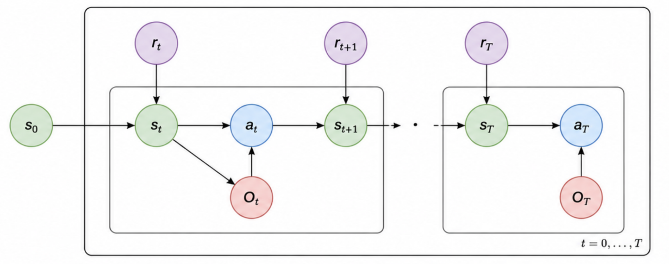
As shown in Figure 1, the reinforcement learning problem can be represented as a directed probabilistic graphical model. The green nodes represent the states \(s_t\), which evolve according to the environment dynamics. The blue nodes represent the actions \(a_t\), sampled from the policy \(\pi(a_t\mid s_t)\). The purple nodes represent the rewards \(r_t\) associated with the state-action pairs.

To formulate control as inference, we augment the MDP with a binary optimality variable \(\calO_t\), shown in red. The event \(\calO_t=1\) indicates that the state-action pair is desirable. We encode the reward through the likelihood of this event:

where \(\alpha>0\) is a temperature parameter.

Assuming that the optimality variables are conditionally independent given the state-action pairs, the likelihood that the entire trajectory is optimal is

For a trajectory

we define the cumulative return as

The optimality likelihood therefore becomes

We can now infer the posterior distribution over trajectories conditioned on the event that the trajectory is optimal. By Bayes rule,

The prior trajectory distribution is induced by the initial-state distribution, the current policy, and the environment dynamics:

where the final action \(a_T\) may be included through an additional policy factor if the trajectory definition contains a terminal action.

Substituting the prior and the optimality likelihood gives

This posterior favors trajectories with high return while retaining the structure imposed by the policy and the environment dynamics. In practice, however, computing this full trajectory distribution is generally intractable. Practical algorithms therefore approximate the inference problem locally at each state.

3. Algorithms as Approximate Inference

Rather than inferring the distribution over complete trajectories, practical RL algorithms use the action-value function \(Q(s,a)\) to summarize the expected future return after taking action \(a\) in state \(s\). This leads to a local target distribution over actions:

The prior \(\pi_{\mathrm{prior}}\) determines which actions are initially considered likely, while the exponential value term increases the probability of actions with high expected return. Different RL algorithms correspond to different choices of prior and different ways of approximating this target distribution.

3.1. Soft Actor–Critic (SAC)

SAC [3] uses maximum-entropy policy improvement. Its actor minimizes the KL divergence between the current policy and a Boltzmann distribution induced by the soft action-value function:

where \(Z(s)\) is the normalizing constant. Expanding this KL divergence gives the maximum-entropy objective shown in equation (1).

3.2. Maximum a Posteriori Policy Optimisation (MPO)

MPO [1] uses the same local inference principle, but explicitly takes the current policy \(\pi_{\mathrm{old}}\) as the action prior. Its target posterior is

where \(\eta>0\) is a temperature parameter. Thus, the inferred distribution favors actions that both have high value and remain close to the current policy.

MPO obtains this distribution by maximizing a local evidence lower bound (ELBO):

Maximizing this ELBO with respect to \(q\) gives the closed-form posterior above. MPO then alternates between two steps:

• E-step: Construct the non-parametric target distribution \(q^*(a\mid s)\) using value-weighted samples from \(\pi_{\mathrm{old}}\).
• M-step: Fit the parametric policy \(\pi_\theta(a\mid s)\) to \(q^*(a\mid s)\) by minimizing \[ D_{\mathrm{KL}} \left( q^*(\cdot\mid s) \,\middle\|\, \pi_\theta(\cdot\mid s) \right), \] while constraining the update relative to \(\pi_{\mathrm{old}}\) through a trust region.

As a result, MPO can be interpreted as coordinate ascent on the ELBO: the E-step infers an improved action distribution, and the M-step projects that distribution back onto the chosen policy class.

References

- A. Abdolmaleki, J. T. Springenberg, Y. Tassa, R. Munos, N. Heess, and M. Riedmiller. Maximum a Posteriori Policy Optimisation. International Conference on Learning Representations, 2018. openreview.net/forum?id=S1ANxQW0b
- S. Levine. Reinforcement Learning and Control as Probabilistic Inference: Tutorial and Review. arXiv:1805.00909, 2018. arxiv.org/abs/1805.00909
- T. Haarnoja, A. Zhou, K. Hartikainen, G. Tucker, S. Ha, J. Tan, V. Kumar, H. Zhu, A. Gupta, P. Abbeel, and S. Levine. Soft Actor-Critic Algorithms and Applications. arXiv:1812.05905, 2019. arxiv.org/abs/1812.05905